We know that equation #1 (from the intro to Laplace transform page) allows us to transform an expression from the time domain to the frequency domain. However, using equation #1 can be cumbersome when the expression is more elaborate than the one found in our rather simplisic example problem. We can reduce our need for equation #1 if we build a basic understanding of some of the known properties of the Laplace transform. We will briefly examine some of the more useful ones in this page. A more comprehensive list of Laplace transform properties can be found in a table such as the one found here.
Linearity Property
Given two time-domain functions: $$ f_1(t)\;and\;f_2(t) $$ ...and their respective Laplace transforms: $$ F_1(s)\;and\;F_2(s) $$ ...the Linearity property states the following:
$$ \mathcal{L}[a_1f_1(t)+a_2f_2(t)] = a_1F_1(s)+a_2F_2(s) \quad,(Eqn\;2a) $$ ...where a1, a2 are constants.
Scaling Property
Given a function f(t) and its transform F(s), consider the following implementation of the definition of the Laplace transform: $$ \mathcal{L}[f(at)] = \int_{0}^{\infty} f(at)e^{-st} dt $$ ...where: $$ a=constant,\;and \; a \gt 0 $$ Using substitution to solve the integral we let: $$ x = at, \; dx = a\;dt $$ $$ t = \frac{x}{a}, \; dt = \frac{dx}{a} $$ We now have: $$ \mathcal{L}[f(at)] = \int_{0}^{\infty} f(x)e^{-s\big( \frac{x}{a} \big)} \frac{dx}{a} $$ $$ \qquad\quad\;\; = \frac{1}{a} \int_{0}^{\infty} f(x) e^{-x\big( \frac{s}{a} \big)} dx \quad,(Eqn\;2b) $$ Now compare equation 2b with the definition of the Laplace transform (equation #1 ):
$$ \mathcal{L}[f(at)] = \frac{1}{a} \int_{0}^{\infty} f(x) e^{-x\big( \frac{s}{a} \big)} dx \;\;\;\Longleftrightarrow\;\;\; \mathcal{L}[f(t)] = F(s) = \int_{0^-}^{\infty} f(t)e^{-st} dt $$
By equating expressions we see that for equation #1, "s" must be replace with "s/a" and "t" must be replaced by "x". This gives us the following expression which is our scaling property:
Scaling property
$$ \mathcal{L}[f(at)] = \frac{1}{a} F\Big(\frac{s}{a}\Big) $$
Time Shift Property
Given a function f(t) and its Laplace transform F(s), consider the following implementation of the definition of the Laplace transform: $$ \mathcal{L}[f(t-t_0)u(t-t_0)] = \int_{0}^{\infty} \Big[f(t-t_0)u(t-t_0) e^{-st}\Big] dt $$ ...where: $$ t_0 \ge 0 $$ Recall the definition of the unit step function (explained in example #1 of the intro to Laplace section.)
$$ u(t-t_0) = \left\{ \begin{array}{ll} 0 & t \lt t_0 \\ 1 & t \ge t_0 \end{array} \right. $$
Illustrated graphically below:
Since we have specified that: $$ t_0 \ge 0 $$ We can see that: $$ u(t-t_0) = 1 $$ Therefor: $$ \mathcal{L}[f(t-t_0)u(t-t_0)] = \int_{0}^{\infty} \Big[f(t-t_0) e^{-st}\Big] dt $$ Using substitution to solve the integral we let: $$ x = t-t_0, \;\;\; dx = 1dt = dt $$ $$ t = x+t_0 $$ We now have: $$ \mathcal{L}[f(t-t_0)u(t-t_0)] = \int_{0}^{\infty} \Big[f(x)e^{-s(x+t_0)}\Big]dx $$ $$ \qquad\qquad\qquad\qquad\;\; = \int_{0}^{\infty} \Big[f(x)e^{-sx}e^{-st_0}\Big]dx $$ $$ \qquad\qquad\qquad\qquad\;\; = e^{-t_0s}\int_{0}^{\infty} \Big[f(x)e^{-sx}\Big]dx $$ ...which is equivalent to the following expression (and is the definition of the Time Shift Property):
Time shift property
$$ \mathcal{L}[f(t-t_0)u(t-t_0)] = e^{-t_0s}F(s) $$ ...where: $$ t_0 = \;"time\;delay" $$
We see that for a function delayed by a certain amount of time (t_0), in order to transform the function to the frequency domain, we first obtain the Laplace transform of the function without the delay and then multiply the result by e^{-t_0 s}
Frequency Shift Property
Given a function f(t) and its Laplace transform F(s), consider the following expression which implements the definition of the Laplace transform: $$ \mathcal{L}[e^{-at}f(t)] = \int_{0}^{\infty} \Big(e^{-at}f(t)e^{-st}\Big)dt $$ $$ \qquad\qquad\;\; = \int_{0}^{\infty} \Big(e^{-t(s+a)}f(t)\Big)dt \qquad,(Eqn\;2c) $$ Let's compare equation 2c to the definition of the Laplace transform (equation #1 ): $$ \mathcal{L}[e^{-at}f(t)] = \int_{0}^{\infty} \Big(e^{-t(s+a)}f(t)\Big)dt \;\;\;\Longleftrightarrow\;\;\; \mathcal{L}[f(t)] = \int_{0^-}^{\infty} f(t)e^{-st} dt = F(s) $$ When comparing the right-hand side of the equal signs for both expressions, notice that equation 2c is the same as equation #1 but with "s" replaced by "s+a". With this knowledge we can now define the frequency shift property as:
Frequency shift property
$$ \mathcal{L}[e^{-at}f(t)] = F(s+a) $$ ...where: $$ s+a = \;"frequency\;shift/frequency\;translation" $$
Time Differentiation Property
Given a function f(t) and its Laplace transform F(s), consider the following expression which implements the definition of the Laplace transform: $$ \mathcal{L}[\frac{df}{dt}] = \int_{0}^{\infty} \Big(\frac{df}{dt}e^{-st}\Big)dt $$
Using integration by parts to solve the integral above: $$\int_{0}^{\infty}u \; dv = uv - \int_{0}^{\infty}v \; du $$ $$ \qquad u=e^{-st} ,\qquad\;\; dv=\frac{df}{dt} $$ $$ \qquad du=-se^{-st}dt ,\;\;\; v = \int_{0}^{\infty} \frac{df}{dt} = f(t)\Big|_0^{\infty} $$
Continuing on: $$ \mathcal{L}[\frac{df}{dt}] = e^{-st}f(t) \Big|_0^{\infty} - \int_{0}^{\infty}[f(t)(-se^{-st})]dt $$ $$ \qquad\;\;\; = \frac{f(t)}{e^{st}}\Big|_0^{\infty} + s\int_{0}^{\infty} f(t)e^{-st}dt $$ $$ \qquad\;\;\; = 0-f(0) + s\int_{0}^{\infty} f(t)e^{-st}dt $$ $$ \qquad\;\;\; = -f(0) + s\int_{0}^{\infty} f(t)e^{-st}dt $$
However, recall the definition of the Laplace transform: $$ \mathcal{L}[f(t)] = F(s) = \int_{0}^{\infty} f(t)e^{-st} dt $$ ...and recognize that we can rewrite our previous expression as:
Laplace transform of the first derivative:
$$ \mathcal{L}[\frac{df}{dt}] = \mathcal{L}[f'(t)] = sF(s)-f(0) \qquad,(Eqn\;2d) $$
Furthermore, if we were to want the Laplace transform pf the second derivative of f(t), we would reiterate equation 2d and get: $$ \mathcal{L}[\frac{d^2f}{dt^2}] = s\mathcal{L}[f'(t)]-f'(0) $$ $$ \qquad\quad\; = s[sF(s)-f(0)]-f'(0) $$ After distributing the "s" term in the above equation we get:
Laplace transform of the second derivative:
$$ \mathcal{L}[\frac{d^2f}{dt^2}] = \mathcal{L}[f''(t)] = s^2F(s)-sf(0)-f'(0) \qquad,(Eqn\;2e) $$
If we were to continue to apply equation 2d we would see that the Laplce transform of the nth derivative of the function f(t) would be defined as follows:
Laplace transform of the nth derivative:
$$ \mathcal{L}[f^n(t)] = s^nF(s)-s^{n-1}f(0)-s^{n-2}f'(0)-...-sf^{n-2}(0)-f^{n-1}(0) \qquad,(Eqn\;2f) $$
Time Integration property
Given a function f(t) and its Laplace transform F(s), the Laplace transform of the integral of f(t) can be found using the definition of the Laplace transform in the following manner: $$ \mathcal{L}\Big[\int_{0}^{t}f(x)dx\Big] = \int_{0}^{\infty} \Big[\int_{0}^{t}f(x)dx\Big]e^{-st}dt $$
In order to use Integration by parts to solve the integral on the right-hand side of the equation, we make the following substitutions: $$ u = \int_{0}^{t}f(x)dx \;\;,\;\; dv = e^{-st} $$ $$ du = f(t)dt \qquad,\;\; v = \frac{-1}{s} e^{-st} $$ Recalling the definition of Integration by parts: $$\int_{}^{}u \; dv = uv - \int_{}^{}v \; du $$ ...we now plug these into our original equation:
$$ \mathcal{L}\Big[\int_{0}^{t}f(x)dx\Big] = \Big[ \int_{0}^{t}f(x)dx \Big]\Big(\frac{-1}{s}e^{-st}\Big)\Big|_0^{\infty}-\int_{0}^{\infty}\frac{-1}{s}e^{-st}f(t) dt $$
$$ \qquad\qquad\;\; = 0-0-\frac{1}{s} \int_{0}^{\infty} f(t)e^{-st}dt$$ $$ \qquad\qquad\;\; = \frac{1}{s}F(s) $$ We can now define the time-integration property for the Laplace transform as:
Time integration property
$$ \mathcal{L}\Big[\int_{0}^{t}f(x)dx\Big] = \frac{F(s)}{s} $$
Frequency Differentiation Property
Recall the definition of the Laplace transform: $$ F(s) = \int_{0}^{\infty}f(t)e^{-st}dt $$ If we were to take the derivative of F(s) with respect to "s" we would have: $$ \frac{dF(s)}{ds} = \int_{0}^{\infty} f(t)(-te^{-st})dt $$ ...which can be rewritten as: $$ \qquad\;\;\; = \int_{0}^{\infty}\Big(-tf(t)\Big)e^{-st} = \mathcal{L}[-tf(t)] $$ This allows us to define the frequency differentiation property as:
Frequency Differentiation Property
$$ \mathcal{L}[tf_1(t)] = \frac{-dF_1(s)}{ds} $$
If we were to take repeated applications of this property we could arrive at a more general expression for the frequency differentiation property:
General expression for the Frequency Differentiation Property
$$ \mathcal{L}[t^nf_1(t)] = (-1)^n \frac{d^nF_1(s)}{ds^n} $$
...where F1(s) is the Laplace Transform of the f(t) part of the expression (excluding the "t" to the nth power part)
Time Periodicity Property
If a function f(t) is periodic, it can be represented as the sum of time-shift functions:
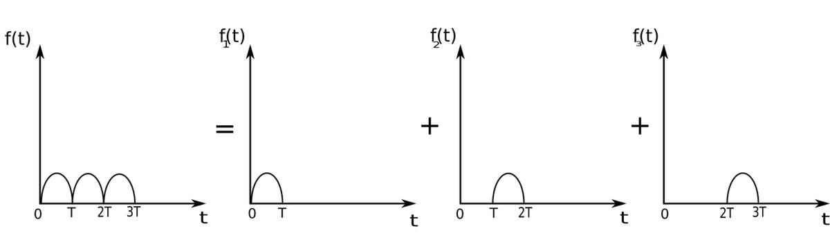
$$ f(t) = f_1(t) + f_2(t) + f_3(t) $$ $$ \quad\;\; = f_1(t) + f_1(t-T)u(t-T) + f_1(t-2T)u(t-2T) + ... \quad(Eqn\;2g) $$ ...where: $$ f_1(t) = \left\{ \begin{array}{ll} f(t) & ,0 \lt t \lt T \\ 0 & ,otherwise \end{array} \right. $$
In order to obtain the Laplace transform of f(t), we proceed to transform each term in equation 2g by means of the Time Shift Property which we derived above:
$$ \mathcal{L}[f(t-t_0)u(t-t_0)] = e^{-t_0s}F(s) $$ ...where: $$ t_0 = \;"time\;delay" $$
...therefore we have: $$ F(s) = F_1(s) + F_1(s)e^{-Ts} + F_1(s)e^{-2Ts} + F_1(s)e^{-3Ts} + ... $$ $$ \qquad = F_1(s)[1 + e^{-Ts} + e^{-2Ts} + e^{-3Ts} + ... ] \quad (Eqn\;2h) $$
...However, note that: $$ 1+x+x^2+x^3 = \frac{1}{1-x} $$ if $$ |x| \gt 1 $$
We can now define the Time Periodicity Property as:
Time Periodicity Property
$$ F(s) = \frac{F_1(s)}{1-e^{-Ts}} $$ ...where F1(s) if the Laplace transform of f(t) defined over its first period only.
Initial and Final Values
From the Laplace transform of a function f(t), it is possible to find f(0) and f(infinity). We begin by recalling the definition of the time-differentiation property as it relates to the 1st derivative (Equation 2d): $$ \mathcal{L}[\frac{df}{dt}] = \mathcal{L}[f'(t)] = sF(s)-f(0) = \int_{0}^{\infty} f'(t)e^{-st} dt $$
If we let "s" approach infinity we get:
$$ \lim_{s\to\infty}\Big[sF(s)-f(0)\Big] = \lim_{s\to\infty}\Big[\int_{0}^{\infty} f'(t)e^{-st} dt\Big] $$
Noting that: $$ \lim_{s\to\infty}\Big[\int_{0}^{\infty} f'(t)e^{-st} dt\Big] = 0 $$ We have:
$$ \lim_{s\to\infty}\Big[sF(s)-f(0)\Big] = 0 $$ Using the properties of limits we can expand the above expression: $$ \lim_{s\to\infty}\Big[sF(s)\Big] - \lim_{s\to\infty}\Big[f(0)\Big] = 0 $$ $$ \lim_{s\to\infty}\Big[sF(s)\Big] - f(0) = 0 $$ By rearranging the above expression we obtain the initial value theorem:
Initial Value Theorem
$$ f(0) = \lim_{s\to\infty}\Big[sF(s)\Big] \qquad ,(Eqn\;2i)$$
If we let "s" approach zero we get:
$$ \lim_{s\to 0}\Big[sF(s)-f(0)\Big] = \int_{0}^{\infty} f'(t)e^{0t} dt $$ $$ \lim_{s\to 0} \Big[sF(s)\Big] - \lim_{s\to 0}\Big[ f(0)\Big] = f(t) \Big|_0^{\infty} $$ $$ \lim_{s\to 0} \Big[sF(s)\Big] - f(0) = f(\infty) - f(0) $$ After canceling like terms in the above expression we obtain the "Final Value Theorem":
Final Value Theorem:
$$ f(\infty) = \lim_{s\to 0} \Big[sF(s)\Big] \qquad ,(Eqn\;2j) $$
Note:
The Final Value Theorem can only be used when the poles of F(s) are all located in the left half of the complex plane. This means that all poles must have real components that are negative. (The exception being when F(s) has a simple pole at s=0). Additionally, the Final Value Theorem does not apply for sinusoidal functions. Such functions oscillate forever and don't have final values. For example: $$ given: \;\;\; f(t) = sin(t) \qquad, \quad F(s) = \frac{1}{s^2+1} $$ $$ poles \; F(s)\; = \pm j $$ Note that these poles are not in the left half of the complex plane.
Continue on to example problems involving the use of Laplace Transform properties...