Determine the Laplace Transform of the following waveform:
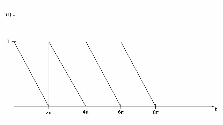
We begin by understanding that this is a periodic waveform with a period of 2pi (T=2pi). With this in mind, the natural next step would be to recognize that the Time Periodicity Property is the method of choice for determining the Laplace Transform of this waveform. The Time Periodicity Property is defined below:
$$ F(s) = \frac{F_1(s)}{1-e^{-Ts}} $$ ...where F1(s) if the Laplace transform of f(t) defined over its first period only.
1) Determine the step function for the 1st period of f(t):
First we define the equation of the line from 0 to 2pi. Notice that within this interval we have the following: $$ slope = m = \frac{-1}{2\pi} $$ $$ y \; intercept = b = 1 $$ Using the formula y=mt+b for a striaght line, we get the following expression: $$ f(t) = \frac{-t}{2\pi} + 1 \qquad,(Eqn\;1)$$ In order to define f(t) over its first period (in terms of a step function), let's recall the definition of the unit step function:
$$ u_c(t) = \left\{ \begin{array}{ll} 0 & t \lt c \\ 1 & t \ge c \end{array} \right. \qquad (Definition \; 1) $$ and is somtimes defined via the following form (which is equivalent to definition #1): $$ u(t-t_0) = \left\{ \begin{array}{ll} 0 & t \lt t_0 \\ 1 & t \ge t_0 \end{array} \right. \qquad (Definition \; 2) $$
Notice that equation #1 is the starting point of f(t) at t = 0. f(t) then decreases (negative slope) unti we reach the end of the period at t = 2pi. We therefore define f(t) over its first period (in terms of a step function) in the following manner: $$ f_1(t) = \Big( 1-\frac{t}{2\pi} \Big) - \Big(1-\frac{t}{2\pi} \Big) u(t-2\pi) $$ $$ f_1(t) = \Big( 1-\frac{t}{2\pi} \Big) + \Big(\frac{t}{2\pi} - 1 \Big) u(t-2\pi) \qquad,(Eqn\;2)$$ By inspection, we recognize that we will need to utilize the Time Shift Property (property #27 in our Laplace Transform table). However, we need to manipulate equation #2 in order to make it resemble a similar form. We can do this by factoring in the following manner:
$$ f_1(t) = 1 - \frac{t}{2\pi} + \frac{1}{2\pi}(t-2\pi) u(t-2\pi) \qquad,(Eqn\;3)$$ Equation #3 is now in a form that will allow us to determine the Laplace transform of f(t) over its 1st period.
2) Determine the Laplace Transform of f(t) defined over its 1st period:
We do this by getting the Laplace transform of equation #3 $$ \begin{align} \mathcal{L}[f_1(t)] &= F_1(s) \\ &= \mathcal{L}[1] - \mathcal{L}\Big[ \frac{t}{2\pi} \Big] + \frac{1}{2\pi}\mathcal{L}[(t-2\pi)u(t-2\pi)] \\ \end{align} $$ For the 1st term of the above expression, we use the 1st property of our Laplace transform table. For the 2nd term, we use the second property of the table. For the 3rd term, we use the Time Shift Property (Property # 27 in the table). Continuing onward we have: $$ \begin{align} F_1(s) &= \frac{1}{s} - \frac{1}{2\pi s^2} + \frac{1}{2\pi}\Big[ e^{-2\pi s} \frac{1}{s^2}\Big] \\ &= \frac{1}{s} - \frac{1}{2\pi s^2} + \frac{e^{-2\pi s}}{2\pi s^2} \\ \end{align} $$
$$ F_1(s) = \frac{2\pi s - 1 + e^{-2\pi s}}{2\pi s^2} \qquad,(Eqn\;4) $$
Once again we recall the Time Periodicity Property: $$ F(s) = \frac{F_1(s)}{1-e^{-Ts}} $$ ...and substitute in equation #4 and the period of 2pi: $$ \begin{align} F(s) &= \frac{2\pi s - 1 + e^{-2\pi s}}{2\pi s^2} \Big( \frac{1}{1-e^{-2\pi s}} \Big) \\ \end{align} $$
$$ F(s) = \frac{2\pi s - 1 + e^{-2\pi s}}{2\pi s^2(1-e^{-2\pi s})} $$