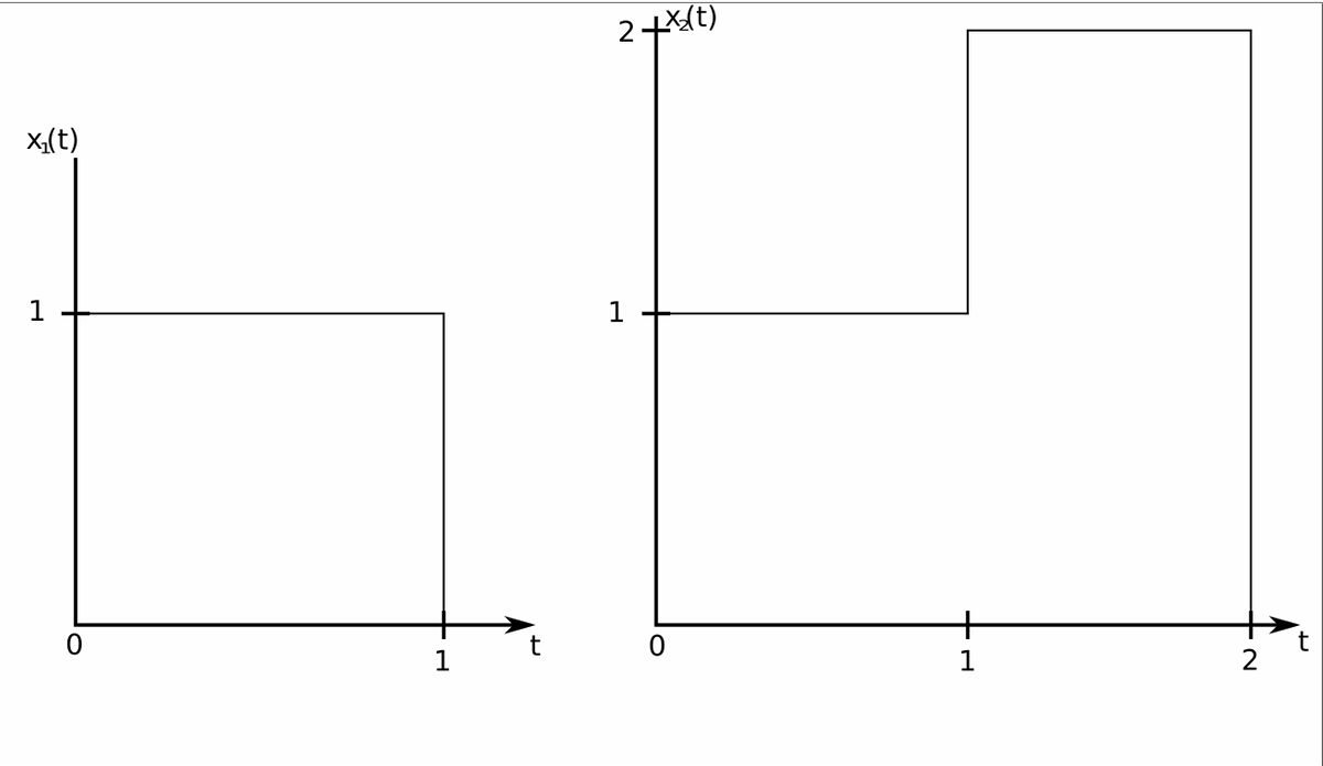
Determine the convolution of the following 2 signals using the graphical method:
We will proceed by following the steps used to evaluate the convolution graphically (outlined in the previous page).
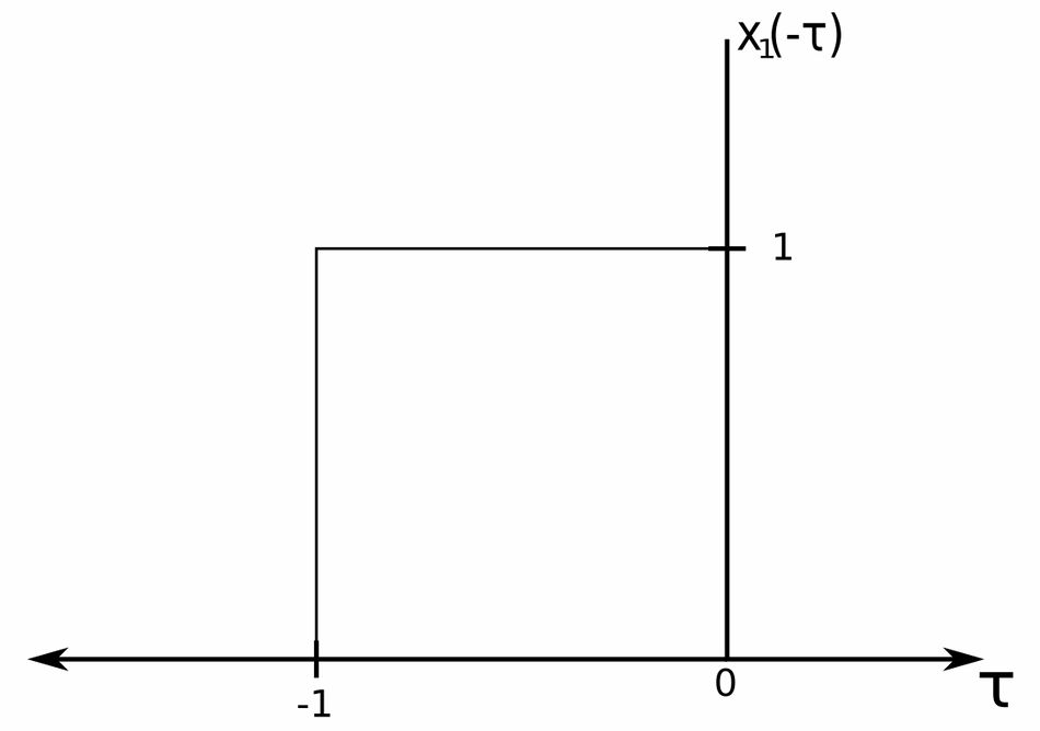
1) Folding: Reflect x_1(t) about the vertical axis
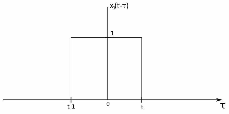
2) Shift:
$$ We \; now \; shift \; x_1(-\tau) \; by \; "t" $$
3 and 4) For different values of "t", multiply the functions and calculate the area under the product
$$ For \; t \lt 0, \; the \; signals \; don't \; overlap $$ $$ \qquad h(t) = 0, \; t \lt 0 $$ $$ $$ $$ For \; 0 \lt t \lt 1 \; we \; have: $$
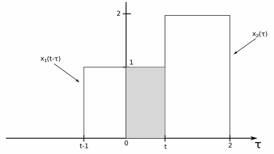
We can see that the two signals overlap between 0 and t. $$ \begin{align} h(t) &= \int_{0}^{t} x_1(t-\tau)x_2(\tau) \; d\tau \\\\ &= \int_{0}^{t} 1(1) \; d\tau \\\\ &= \tau \Big|^t_{0} \\\\ &= t-0 \\\\ \end{align} $$
$$ h(t) = t \; , \;\;\; 0 \lt t \lt 1 $$
$$ For \; 1 \lt t \lt 2 \; we \; have: $$
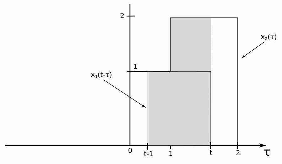
The signals overlap from "t-1" to "t". However, we will break this into two parts since: $$ x_1(t-\tau) = 1 \; , \; from \; (t-1) \; to \; t $$ $$ \begin{align} x_2(\tau) &= 1 \; , \; from \; (t-1) \; to \; 1 \\ &= 2 \; , \; from \; 1 \; to \; t \end{align} $$ ...therefore, we have: $$ \begin{align} h(t) &= \int_{t-1}^{1}1(1)\;d\tau + \int_{1}^{t}1(2)\;d\tau \\\\ &= \tau \Big|^1_{t-1} + 2\big[ \tau \big] \Big|^t_{1} \\\\ &= 1-(t-1) + 2(t-1) \\\\ &= 2-t+2t-2 \end{align} $$
$$ h(t) = t \; , \;\;\; 1 \lt t \lt 2 $$
$$ For \; 2 \lt t \lt 3 \; we \; have: $$
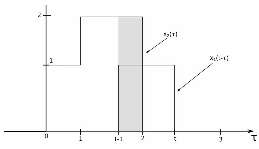
The signals overlap from (t-1) to 2. Therefore we have the following: $$ \begin{align} h(t) &= \int_{t-1}^{2}2(1)\;d\tau \\\\ &= 2\big[\tau\big] \Big|^{2}_{t-1} \\\\ &= 2[2-(t-1)] \\\\ &= 2(3-t) \end{align} $$
$$ h(t) = 6-2t \; , \;\;\; 2 \lt t \lt 3 $$
$$ For \; t \gt 3, \; the ;\ signals \; don't \; overlap $$ $$ \qquad h(t) = 0, \; t \gt 3 $$
Our final answer for the convolution is
$$ h(t) = \left\{ \begin{array}{ll} t \;\;,\;\; & 0 \lt t \lt 2 \\ 6-2t \;\;,\;\; & 2 \lt t \lt 3 \end{array} \right. $$
Which (graphically speaking) would look something like what we have below:
Continue on to example problem #2 involving the graphical approach to solving the convolution integral...