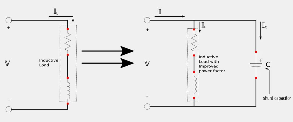
In terms of real-world AC power analysis, many household and industrial loads are inductive in nature. As a result, they operate at a low (lagging) power factor. Towards the end of our introduction to the concept of the power factor (under the heading "some points to consider"), it was mentioned that given two loads with equal power transfers, the load with a lower power factor draws more current and is less efficient than the load with a higher power factor. The power factor of an inductive load is corrected (improved) by placing a capacitor (often called a "shunt capacitor") in parallel with the load.
The change in properties to the circuit (due to the capacitor) are represented in the following phasor diagram:
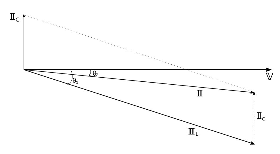
We see that the "improved" circuit has a decreased angle between supplied voltage and current. Since: $$ \theta_v - \theta_i = power \; factor \; angle $$ and $$ \cos(\theta_v - \theta_i) = power \; factor$$ ...we see that a smaller phase angle results in a higher (improved) power factor. We also notice that the magnitudes of the vectors are different. Specifically we see that for the same supplied voltage, the original circuit draws more current than the improved circuit. $$ \mathbb{I}_L \gt \mathbb{I} $$ Therefore, by selecting the appropriate size capacitor, the circuit can be made to be more "in-phase" with the voltage (potentially completely in phase resulting in a unity power factor.) We can also use the power triangle to show the effects of the parallel capacitor:
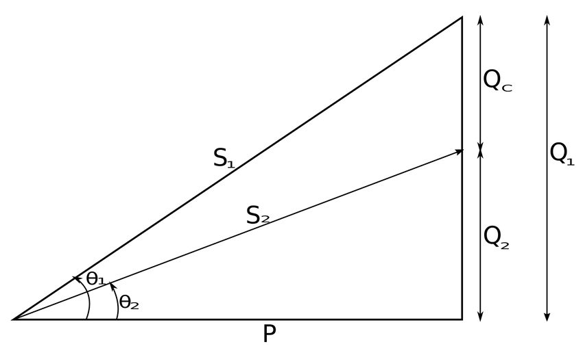
...where: $$ \mathbb{S}_1 = complex \; power \; for \; original \; circuit $$ Recall that: $$ P_f = \cos(\theta_v - \theta_i) $$ For the original (uncorrected) circuit, let: $$ \theta_1 = P_f \; angle \; for \; original \; circuit. $$ We also know that power can be expressed as the following: $$ P = SP_f $$ Therefore, the power for the original circuit is: $$ P = S_1 \cos(\theta_1) $$ Recall our previously defined expressions for reactive power, and recognize that the reactive power for the uncorrected circuit is defined as: $$ Q_1 = S_1 \sin(\theta_1) $$ Using simple trigonometry on our power triangle (up above), we can also define Q1 as: $$ Q_1 = P\tan(\theta_1) \qquad(Eqn \; 1) $$ Our goal is to increase the power factor from: $$ \cos(\theta_1) \rightarrow \cos(\theta_2)$$ ...without altering the real power (P) of the circuit. From our power triangle we see that the "new" reactive power for the corrected circuit becomes: $$ Q_2 = S_2\sin(\theta_2) = P\tan(\theta_2) \qquad(Eqn \;2) $$ Now let Qc equal the reduction of reactive power due to the shunt capacitor placed in parallel with the load: $$ Q_C = Q_1-Q_2 $$ Substituting equations 1 and 2 into the above expression gives us: $$ Q_C = P\tan(\theta_1) - P\tan(\theta_2) $$ $$ Q_C = P[\tan(\theta_1) - \tan(\theta_2)] \qquad(Eqn \; 3) $$ Now, recall the following expression for impedance: $$ \mathbb{Z} = R+jX $$ For a capacitor, its nature is entirely reactive (R=0) and associated with a negative "j". Thus we have: $$ \mathbb{Z}_C = -jX_C \qquad(Eqn \; 4)$$ Now recall our second expression for complex power (found in the intro to complex power page): $$ \mathbb{S} = P+jQ = \frac{V^2_{rms}}{\mathbb{Z}*} $$ For the capacitor in our corrected circuit, we determined a value for its impedance when we derived equation #4. Therefore the complex conjugate of that impedance is: $$ \mathbb{Z^*}_C = jX_C $$ Our expression for the complex power of the capacitor now becomes: $$ \mathbb{S}_C = \frac{V^2_{rms}}{jX_C} = \frac{-j \; V^2_{rms}}{X_C} \qquad(Eqn \; 5)$$
Recall that: $$ Q = I_m \{ \mathbb{S} \} $$
We now can define the reactive power of the shunt capacitor as: $$ Q_C = I_m \{ \mathbb{S}_C \} = \frac{V^2_{rms}}{X_C} $$
Recall that: $$ X_C = \frac{1}{\omega C} $$
The reactive power of the shunt capacitor now becomes: $$ Q_C = V^2_{rms} \omega C $$ ...and through simple algebra, the value of the shunt capacitor becomes: $$ C = \frac{Q_C}{\omega V^2_{rms}} $$ We now substitute equation #3 into the above expression and get:
The value of the shunt capacitance required to correct the power factor to unity (for an inductive load):
$$ C = \frac{P[\tan(\theta_1) - \tan(\theta_2)]}{\omega V^2_{rms}} $$
Correcting a Capacitive Load:
While it is more common to apply power factor correction to inductive loads, what happens if we want to correct a capacitive load? In this case, instead of placing a capacitor in parallel with the load, we place an inductor in parallel in order to correct the leading (as opposed to lagging) power factor. The general approach to deriving the value for the inductor is similar to the approach used above for the capacitor value with the obvious difference being the expressions for the impedance and reactance of an inductor. I won't go through the derivation here but if you do you will get the following:
The value of the parallel inductor required to correct the power factor to unity (for a capacitve load):
$$ L = \frac{V^2_{rms}}{\omega Q_L} = \frac{V^2_{rms}}{\omega [P(\tan \theta_1 - \tan \theta_2)]} $$
We will now go ahead and look at some example problems involving power factor correction for inductive loads.
Continue on to Power factor correction example problem...