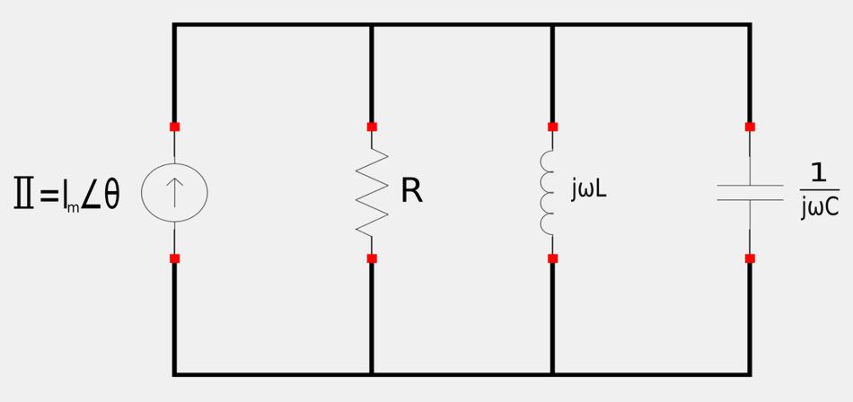
We will now proceed to develop an understanding of resonance in parallel RLC circuits. We will use a similar approach as we did with Series Resonance, but rather than utilizing the concept of impedance, we will use the concept of admittance. Consider the following circuit with labeled impedance values:
Admittance
Recall that admittance is the inverse of impedance: $$ \mathbb{Y} = \frac{1}{\mathbb{Z}} = \frac{\mathbb{I}}{\mathbb{V}} $$ For the individual components of our parallel RLC circuit we have: $$ \mathbb{Y}_R = \frac{1}{R} $$ $$ \mathbb{Y}_L = \frac{1}{j\omega L} $$ $$ \mathbb{Y}_C = j\omega C $$ To find the input admittance of the circuit we use the inverse of the rule for impedances in parallel: $$ \mathbb{Y}_{in} = \mathbb{Y}_R + \mathbb{Y}_L + \mathbb{Y}_C $$ $$ \quad\;\; = \frac{1}{R} + \frac{1}{j\omega L} + j\omega C $$ $$ \quad\;\; = \frac{1}{R} + j\omega C - \frac{j}{\omega L} $$ $$ \mathbb{Y}_{in} = \frac{1}{R} + j(\omega C - \frac{1}{\omega L}) \qquad,(Eqn\;1) $$ Recall that admittance can be expressed in to the following form: $$ \mathbb{Y} = G + jB $$ ...where: $$ G = R_e \{ \mathbb{Y} \} = conductance $$ $$ B = I_m \{ \mathbb{Y} \} = susceptance $$
Resonant Frequency
For our parallel RLC circuit, resonance occurs when: $$ I_m \{ \mathbb{Y}_{in} \} = 0 $$ In regards to equation #1, this means that: $$ \omega C - \frac{1}{\omega L} = 0 $$ Just as with series resonance, the value of omega that satisfies the above equation is the resonant frequency: $$ \omega_o C = \frac{1}{\omega_o L} $$
$$ \omega_0 = \frac{1}{\sqrt{LC}} = resonant\;frequency\;in\;\frac{rad}{s} $$ or $$ f_o = \frac{1}{2\pi\sqrt{LC}} = resonant\;frequency\;in\;Hz $$
Note that the expressions for the resonant frequency of a parallel RLC circuit are the same as for a series RLC circuit.
Notable characteristics of resonant frequency in parallel RLC circuit
- At resonance, inductor and capacitor current can be much more than source current: $$ I_L = \frac{I_m R}{\omega_o L}=QI_m \qquad, I_C = \omega_oCI_mR=QI_m $$ Where Q = quality factor
- At resonance, the circuit is purely condictive (susceptance = 0) and no current flows through the inductor or capacitor. The parallel "LC" part of the circuit is an open circuit and the entire current flows through the resistor.
Much of the technique used to derive expressions for half-power frequencies, Bandwidth and Quality factor is similar to what we did in the introduction page for Series Resonance. The following expressions are simply listed below:
Half-power frequencies:
$$ \omega_1 = -\frac{1}{2RC} + \sqrt{\Big( \frac{1}{2RC} \Big)^2 + \frac{1}{LC}} $$ $$ \omega_2 = \frac{1}{2RC} + \sqrt{\Big( \frac{1}{2RC} \Big)^2 + \frac{1}{LC}} $$
Bandwidth:
$$ B = \omega_2 - \omega_1 = \frac{1}{RC} $$
Quality factor:
$$ Q = \frac{\omega_o}{B} = \omega_o RC = \frac{R}{\omega_o L} $$
Relating half-power frequencies to Quality Factor:
$$ \omega_1 = \omega_o \sqrt{1+ \Big( \frac{1}{2Q} \Big)^2} - \frac{\omega_o}{2Q} $$ $$ \omega_2 = \omega_o \sqrt{1+ \Big( \frac{1}{2Q} \Big)^2} + \frac{\omega_o}{2Q} $$
High-Q circuits:
$$ Q \geq 10 $$ $$ \omega_1 \approx \omega_o - \frac{B}{2} $$ $$ \omega_2 \approx \omega_o + \frac{B}{2} $$
Continue on to parallel resonance (example problem #1)...