When we discuss the natural response of a series RLC circuit, we are talking about a series RLC circuit that is driven solely by the energy stored in the capacitor and inductor (Also described as being "source-free"). Let's consider such a circuit (shown below), where the current (i) is assumed to travel clockwise around the circuit.
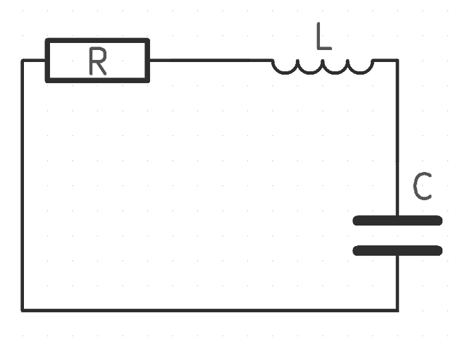
Also, recall the definitions for the voltage across a resistor (R), inductor (L) and capacitor (C):
$$V_R = iR $$
$$V_L = L\frac{di}{dt} $$
$$V_C = \frac{1}{C} \int_{}^{} i \; dt $$
By using Kirchoff's Voltage Law (KVL) and traveling clockwise around the circuit (starting at resistor), we obtain the following equation when using the above definitions.
$$Ri + L\frac{di}{dt} + \frac{1}{C} \int_{}^{} i \; dt = 0 $$
If we take the derivative of the above equation we get:
$$R\frac{di}{dt} + L\frac{d^2i}{dt^2} + \frac{1}{C} \; i = 0 $$
By rearranging the equation and dividing by L we obtain:
$$\frac{d^2i}{dt^2} + \frac{R}{L} \frac{di}{dt} + \frac{1}{LC} \; i = 0 $$
...also written as:
$$i'' + \frac{R}{L} \; i' + \frac{1}{LC}\;i = 0 \qquad ,(Eqn \;1)$$
Equation #1 is a 2nd order differential equation that models a "source-free" RLC circuit or the "natural response" of an RLC circuit. If you have previously visited the Second Order Differential Equations page, you will recognize that this 2nd order Homogeneous equation can be solved by assuming that solutions to the equation ,i(t), are of the following form:
$$i = e^{st} $$
...and where the 1st and 2nd derivatives of i(t) are the following:
$$i' = se^{st} $$
$$i'' = s^2e^{st} $$
If we plug the above 3 expressions into equation #1, we get:
$$s^2e^{st} + \frac{R}{L}se^{st} + \frac{1}{LC}e^{st} = 0 $$
...and dividing through by e^(st):
$$s^2 + \frac{R}{L}s + \frac{1}{LC} = 0 \qquad ,(Eqn \;2)$$
You may recognize equation #2 as being the "characteristic equation" of equation #1 and just as the Second Order Differential Equations page shows us, we can use the quadratic formula to find the roots (values of s) for the characteristic equation:
$$s = \frac{-b \pm \sqrt[]{b^2-4ac}}{2a} \qquad ,(Quadratic \;formula)$$
$$s = \frac{\frac{-R}{L} \pm \sqrt[]{\frac{R^2}{L^2} - \frac{4}{LC}}}{2} $$
$$s = \frac{-R}{2L} \pm \sqrt[]{\frac{R^2}{2L^2} - \frac{4}{LC}} \qquad ,(Eqn \;3)$$
We should note here that it is common to see the following substitution for the above equation where:
$$\alpha = \frac{R}{2L} = \; "neper \; frequency"$$
and
$$\omega_0 = \frac{1}{\sqrt{LC}} = \; "resonant \; frequency" \; or \; "undamped \; natural \; frequency"$$
With this in mind, equation #3 gives us roots of the characteristic equation (equation #2) represented by:
$$s_1 = -\alpha + \sqrt{\alpha^2 - \omega_0^2} $$
$$s_2 = -\alpha - \sqrt{\alpha^2 - \omega_0^2} $$
...and just as in the Second Order Differential Equations page, there are three possible scenarios based on the roots we obtain.
Case #1: two unique real roots (s1 != s1)
The "Over-damped Case":
Know that for the purposes of evaluating source-free RLC circuits, the roots will also turn out to be negative numbers in addition to being unique and real. Such a scenario occurs when:
$$\frac{R}{2L} \gt \frac{1}{\sqrt{LC}} \;, \quad or\; \alpha \gt \omega_0 $$
we get this when the capacitor value is as follows:
$$C \gt \frac{4L}{R^2} $$
For the over-damped case, the solution to the original differential equation for a source-free RLC circuit (equation #1) will be of the following form:
$$i(t) = Ae^{s_1t} + Be^{s_2t} $$
You may find helpful information in solving the differential equation for the over-damped case here
Case #2: two real repeated roots (s1 = s1)
The "Critically Damped Case":
Case #2 occurs when:
$$\frac{R}{2L} = \frac{1}{\sqrt{LC}} \;, \quad or\; \alpha = \omega_0 $$
..and when we have a capacitor value of:
$$C = \frac{4L}{R^2} $$
As you work through the math of such a case you will find that you get roots that resemble the following:
$$s_1 = s_2 = \frac{-R}{2L} = -\alpha $$
Once again, you can refer to this section of the 2nd order differential equations tutorials, where you will find information on how to use "D'Alembert's Procedure" to get a second unique solution to the original equation.
For the critically-damped case, the final solution to the original differential equation for a source-free RLC circuit (equation #1) will be of the following form:
$$i(t) = Ate^{-\alpha t} + Be^{-\alpha t} \quad ,\; where \; \alpha=\frac{R}{2L} $$
The maximum value of i(t) will also be found to occur where:
$$t = \frac{1}{\alpha} = \frac{2L}{R} $$
...from which point it gradually decays to zero.
Case #3: complex roots
The "Under-damped Case":
Case #3 occurs when:
$$\frac{R}{2L} \lt \frac{1}{\sqrt{LC}} \;, \quad or\; \alpha \lt \omega_0 $$
..and when we have a capacitor value defined as:
$$C \lt \frac{4L}{R^2} $$
The roots of the characteristic equation will be complex and of the form:
$$s_{1,2} = -\alpha \pm j \omega_d $$
...where:
$$j = \sqrt{-1} $$
$$\omega_d = \sqrt{\omega_0^2 - \alpha^2} $$
Helpful information on how to solve differential equations with complex roots that resemble the under-damped case can be found here
Lastly, final solutions to such a case will be of the form:
$$i(t) = Ae^{-\alpha t}cos(t\sqrt{\omega_0^2 - \alpha^2}) + Be^{-\alpha t} sin(t\sqrt{\omega_0^2 - \alpha^2})$$
Next, we will use all of the above to solve for an unknown in an actual circuit.
Continue on to RLC series circuit example #1