When we discuss the natural response of a parallel RLC circuit, we are talking about a parallel RLC circuit that is driven solely by the energy stored in the capacitor and inductor (Also described as being "source-free"). Let's consider such a circuit (shown below)
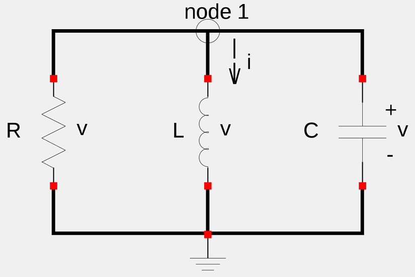
Also, recall the definitions for the current through a resistor (R), inductor (L) and capacitor (C):
$$I_R = \frac{V}{R} $$
$$I_L = \frac{1}{L} \int_{}^{} v \; dt $$
$$I_C = C \frac{dv}{dt} $$
We will use Kirchoff's Current Law (KCL) at node 1:
$$\frac{v}{R} + \frac{1}{L} \int {}^{}v \; dt + C \frac{dv}{dt} = 0 $$
If we take the derivative of the above equation we get:
$$\frac{1}{R} \frac{dv}{dt}+ \frac{1}{L} v + C \frac{d^2v}{dt^2} = 0 $$
By rearranging terms and dividing through by C, we get:
$$v'' + \frac{1}{RC}v' + \frac{1}{LC}v = 0 \qquad Eqn \;1 $$
Just as with source-free series RLC circuits, we will use the techniques discussed in the 2nd order homogeneous differential equations tutorial to solve eqn #1 (which models the capacitor voltage of our source-free parallel RLC circuit). We will use a substitution that assumes v(t) takes the following form:
$$v = e^{st} $$
...with the following 1st and 2nd derivatives;
$$v' = se^{st} $$
$$v'' = s^2e^{st} $$
By substituting the above 3 expressions into equation 1, we get:
$$ s^2e^{st} + \frac{1}{RC}se^{st} + \frac{1}{LC}e^{st} = 0 $$
Dividing through by the exponential term:
$$ s^2 + \frac{1}{RC}s + \frac{1}{LC} = 0 \qquad Eqn \;2 $$
Equation #2 is our "characteristic equation" and by use of the quadratic formula can be found to have the following roots:
$$s_{1,2} = - \frac{1}{2RC} \pm \sqrt{(\frac{1}{2RC})^2 - \frac{1}{LC}} $$
Just as with source-free series RLC circuits, it is common to see a simplification/substitution of terms that are labeled as the "neper" and "resonant" frequencies where:
$$\alpha = \frac{1}{2RC} = neper \; frequency $$
$$\omega_0 = \frac{1}{\sqrt{LC}} = resonant \; frequency $$
...which means that we can express the roots of our characteristic equation as:
$$s_{1,2} = - \alpha \pm \sqrt{\alpha^2 - \omega_0^2} $$
We are once again left with three possible outcomes based on the roots of our characteristic equation:
Case #1: s1 != s2, (2 unique, real roots)
The Overdamped Case
This occurs when:
$$\alpha \gt \omega_0 $$
or:
$$\frac{1}{2RC} \gt \frac{1}{\sqrt{LC}} $$
..which means that the value of our inductor coincides with the following:
$$L \gt 4R^2C $$
Also note that in such a case the roots will be negative (in addition to being unique and real). Values for capacitor voltage (as well as resistor and inductor voltage since all 3 components are in parallel) will be of the form:
$$v(t) = Ae^{s_1 t} + Be^{s_2 t} $$
You may find helpful information in solving the differential equation for the over-damped case here
Case #2: s1 = s2, (2 real repeated roots)
The Critically Damped Case
This occurs when:
$$\alpha = \omega_0 $$
or:
$$\frac{1}{2RC} = \frac{1}{\sqrt{LC}} $$
..which means that the value of our inductor coincides with the following:
$$L = 4R^2C $$
You can refer to this section of the 2nd order differential equations tutorials, where you will find information on how to use "D'Alembert's Procedure" to get a second unique solution to equation #1. After doing so you will obtain a value for the capacitor voltage that has the form of:
$$v(t) = Ae^{-\alpha t} + Bte^{-\alpha t} $$
Case #3: (complex roots)
The Under-damped Case
This occurs when:
$$\alpha \lt \omega_0 $$
or:
$$\frac{1}{2RC} \lt \frac{1}{\sqrt{LC}} $$
..which means that the value of our inductor coincides with the following:
$$L \lt 4R^2C $$
The roots of the characteristic equation will be complex and of the form:
$$s_{1,2} = -\alpha \pm j \omega_d $$
...where:
$$j = \sqrt{-1} $$
$$\omega_d = \sqrt{\omega_0^2 - \alpha^2} $$
Helpful information on how to solve differential equations with complex roots that resemble the under-damped case can be found here. Capacitor voltage values will be of the form:
$$v(t) = Ae^{-\alpha t}cos(\omega_d t) + Be^{-\alpha t}sin(\omega_d t) $$
In the next page of this section we will work through an actual example and determine the natural response of a parallel RLC circuit.
Continue on to RLC parallel circuit example #1