Quadratic Pole
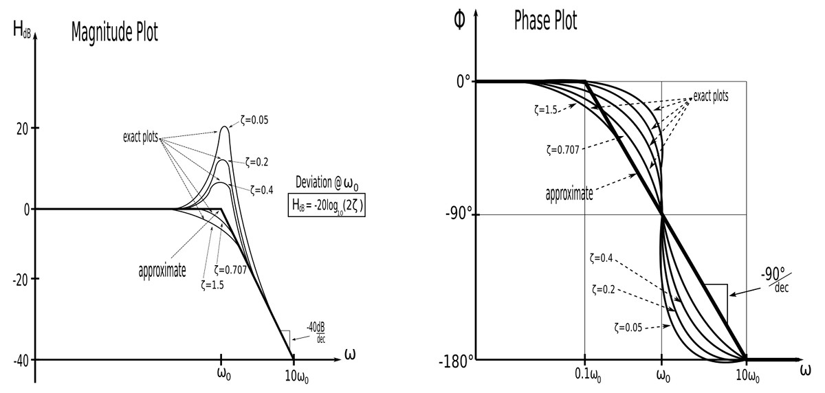
A quadratic pole has the following form: $$ \frac{1}{1+j2\zeta\Big(\frac{\omega}{\omega_0}\Big)+\Big( \frac{j\omega}{\omega_0} \Big)^2} \qquad,where\;\zeta = damping\;coefficient $$ $$ \qquad\qquad\qquad\qquad\qquad\qquad, \omega_0 = corner\;frequency $$ or: $$ \frac{1}{1+2\zeta\Big(\frac{s}{\omega_0}\Big)+\Big( \frac{s}{\omega_0} \Big)^2} \qquad,where\;s=j\omega $$ The magnitude of the quadratic pole is defined as: $$ magnitude = H_{dB} = -20log_{10}\Big| \frac{1}{1+j2\zeta\Big(\frac{\omega}{\omega_0}\Big)+\Big( \frac{j\omega}{\omega_0} \Big)^2}\Big|$$ $$ phase = \phi = \tan^{-1}\Big( \frac{2\zeta(\frac{\omega}{\omega_0})}{1-(\frac{\omega}{\omega_0})^2} \Big) $$ The magnitude and phase plots appear as follows:
Quadratic Zero
As you might expect, the plots for a Quadratic Zero are simply the plots of the Quadratic Pole reflected about the horizontal axis.
Bode Plots and Precision
Notice that the deviation between the exact and approximate plots depends on the damping coefficient (zeta). For the magnitude plot, the deviation at the corner frequency is defined as: $$ H_{deviation \; in \; dB} = -20\log_{10}(2\zeta) $$ For the phase plot, the value of zeta can be used adjust slope for the quadratic factor. Essentially, we can use the value of the damping coefficient (zeta) to correct our straight-line approximation plots and give them more precision. Keep in mind however that they will still be approximations. If precise values are needed along the curve you would be better off constructing the Bode Plot via software such as Maple or Matlab.
Now it's time to take a look at some examples of Bode Plots.
Continue on to Bode Plot (example #1)...