Sketch the Bode plots for the following transfer function:
$$ H(s) = \frac{0.1(s+1)}{s^2(s+10)} $$
Rewrite the expression in a recognizable form for zeros and poles:
We recognize that the transfer function contains a repeated pole at the origin a simple zero and a simple pole. We begin by rewriting it in a more standard form: $$ H(s) = \frac{0.1(1+\frac{s}{1})}{10s^2(1+\frac{s}{10})} $$
$$ H(s) = \frac{0.01(1+\frac{s}{1})}{s^2(1+\frac{s}{10})} \qquad,(Eqn\;1) $$
Determing magnitude via logarithms
If we substitute "jw" for "s" in equation #1 we get: $$ \mathbb{H}(j\omega) = \frac{0.01(1+\frac{j\omega}{1})}{(j\omega)^2(1+\frac{j\omega}{10})} $$ $$ \qquad \;\;\; = \frac{0.01(1+j\omega)}{(j\omega)^2(1+0.1j\omega)} \qquad,(Eqn\;2) $$ Recall that the gain/magnitude of a transfer function is defined as: $$ H_{dB} = 20 \log_{10}|\mathbb{H}(j\omega)| $$ If we apply this expression to equation #2 and use the properties of logarithms we get the following expression:
$$ H_{dB} = 20\log_{10}0.01+20\log_{10}|1+j\omega|-20\log_{10}|(j\omega)^2|-20\log_{10}|1+0.1j\omega| $$ $$ H_{dB} = -40 + 20\log_{10}\sqrt{1+\omega^2} - 20\log_{10}\omega^2 - 20\log_{10}\sqrt{1+0.01\omega^2} $$
$$ H_{dB} = -40 + 10\log_{10}(1+\omega^2) - 40\log_{10}\omega - 10\log_{10}(1+0.01\omega^2) \qquad,(Eqn\;3) $$
Sketch the magnitude plot by examining equation #1
From equation #1 we see that we have the following corner frequencies: $$ \omega_0 = +1, -10 $$ ...where the "+" and "-" are simply a means of designating a zero (positive sign) and a pole (negative sign). We sketch the magnitude plot by examining each of the transfer function factors in order of increasing corner frequencies.
First Factor (constant term):
In equation #1 we see that the first factor is the constant 0.01. Recalling the section on Bode plots and constant factors, we know that the magnitude for the constant factor in our transfer function is: $$ H_{db} = 20\log_{10}0.01 = -40 dB $$ You might think that we would sketch a straight horizontal line at -40 dB from a frequency of 0 rad/sec until 0.1 rad/s, but remember that the horizontal axis is logarithmic and for that reason 0 rad/sec is never included. Many Bode plots begin the horizontal axis at 0.1 ( or 10^-1) rad/sec. Depending on the factors of the transfer function and the corner frequencies, it could begin at a higher frequency. Nevertheless, the magnitude of the constant will be combined with the next factor. Since the next factor (in order of corner frequencies) is the repeated pole at the origin, we carry the -40 db magnitude over to 0.1 rad/sec.
Second Factor (repeated poles at origin):
The second factor is a repeated Pole at the Origin. By "repeated" we mean there are two poles at the origin due to the squared term: $$ \frac{1}{s^2} = \frac{1}{s} \times \frac{1}{s}$$ The straight-line magnitude plot of a pole at the origin has a slope of -20 dB/decade. However, due to the squared term, we have two of them which means the slope becomes -40 dB/decade. Also a single pole at the origin begins at 20dB. Once again, we have two poles at the origin which means we would begin at 40dB. However, we must not forget about the constant term discussed above. The magnitude of this constant is -40dB and when we combine it with the starting 40dB of the repeated pole we get 0dB. This means we start at 0dB and draw a straight line with a slope of -40dB/decade until we hit the first corner frequency of 1 rad/sec. $$ slope = -40\frac{dB}{dec} \qquad,(0 \leq \omega \leq 1)$$
Third Factor (simple zero):
The corner frequency of 1 rad/sec is associated with the Simple Zero: $$ 1+\frac{s}{1} $$ The straight-line magnitude plot of a simple zero has a slope of 20 dB/decade but this is combined with the previous slope of -40 dB/decade from the repeated pole at the origin. This gives us a net slope of -20 dB/decade in between the corner frequencies: $$ slope = \Big( -40\frac{dB}{dec} + 20\frac{dB}{dec}\Big) = -20\frac{dB}{dec} \qquad,(1 \leq \omega \leq 10)$$ Therefore we draw a straight line with a slope of -20 dB/decade from 1 rad/sec to the next corner frequency (10rad/sec).
Fourth Factor (simple pole):
The corner frequency of 10 rad/sec is associated with the Simple Pole: $$ \frac{1}{1+\frac{s}{10}} $$ The straight-line magnitude plot of a simple pole has a slope of -20dB/decade, but this is combined with the previous slope of -20dB/decade. This gives us a net slope of -40dB/decade for frequencies greater than 10 rad/sec: $$ slope = \Big( -20\frac{dB}{dec} - 20\frac{dB}{dec}\Big) = -40\frac{dB}{dec} \qquad,(\omega \gt 10\frac{rad}{s})$$ Therefore we draw a straight line with a slope of -40dB/decade from 10 rad/sec onwards.
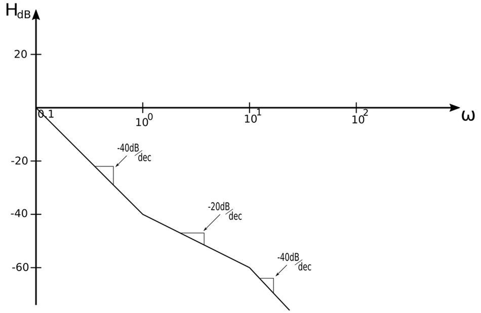
Straight-line approximation for Bode magnitude plot:
After examining the four factors of the transfer function in the manner described above, the final straight-line approximation of the Bode magnitude plot appears as follows
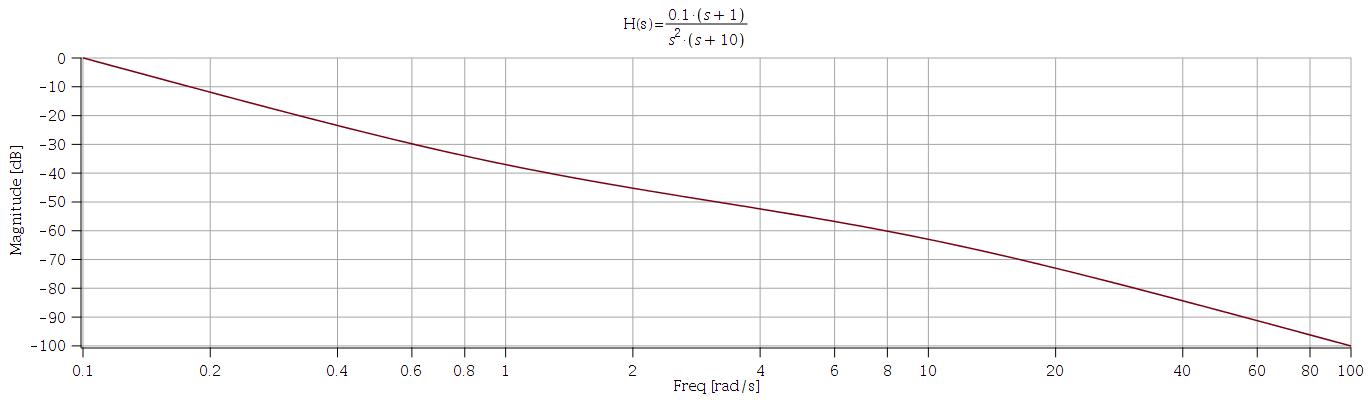
Exact Bode Magnitude Plot:
Below we see the exact Bode magnitude plot (achieved via software):
Determine phase using concept of phasors
Recall equation #2: $$ \mathbb{H}(j\omega) = \frac{0.01(1+j\omega)}{(j\omega)^2(1+0.1j\omega)} \qquad,(Eqn\;2) $$ Also, recall that we can determine the phase angle of any complex phasor quantity by recognizing that: $$ \phi = \tan^{-1} \Big( \frac{imaginary\;part}{real\;part} \Big) $$ Applying this to equation #2 gives us:
$$ \phi = -180^{\circ} + \tan^{-1}(\omega) - \tan^{-1}(0.1\omega) $$
The -180 degrees comes from the repeated poles at the origin which have constant phase angles of -90 degrees each.
Sketch the phase plot
Simple Zero
Once again, when sketching the phase plot, it is important to remember that for factors of the transfer function not at the origin, the slopes of those factors affect the overall plot over a range of frequency values starting at one decade before to one decade after their respective corner frequencies. Consider the corner frequency of 1 rad/sec associated with the Simple Zero of our transfer function: $$ 1+\frac{s}{1} $$
- For corner frequency of 1 rad/s:
- $$ 1 \; decade \; before = 0.1 \frac{rad}{s} $$
- $$ 1 \; decade \; after = 10 \frac{rad}{s} $$
A single Simple Zero has a straight-line phase plot with a slope of +45 deg/decade. Therefore, the simple zero in our transfer function imparts a slope of: $$ +45\frac{deg}{dec} \qquad,over \; the \; range\;(0.1 \leq \omega \leq 10 ) $$
Simple Pole
Now let's look at the corner frequency of 10 rad/sec associated with the Simple Pole of our transfer function: $$ \frac{1}{1+\frac{s}{10}} $$
- For corner frequency of 10 rad/s:
- $$ 1 \; decade \; before = 1 \frac{rad}{s} $$
- $$ 1 \; decade \; after = 100 \frac{rad}{s} $$
A single Simple Pole has a straight-line phase plot with a slope of -45 deg/decade. Therefore, the simple pole in our transfer function imparts a slope of: $$ -45\frac{deg}{dec} \qquad,over \; the \; range\;(1 \leq \omega \leq 100) $$
Constant term and repeated pole at origin
The constant factor of our transfer function is: $$ 0.01 $$ As explained in the section on Bode plots and constant factors, the constant term imparts a phase angle of zero degrees. The repeated Pole at the Origin imparts a constant phase angle of -90 degrees for each individual pole. Since there are effectively two poles at the origin, this implies a phase angle of -180 degrees. The combination of the 0 degrees for the constant and -180 degrees for the repeated pole at the origin imparts a phase angle of -180 degrees. Once again, you may be tempted to draw a horizontal line at -180 degrees from w=0 up till our first frequency of interest (w=0.1). Remember however that the horizontal axis is logarithmic and as such we never include w=0 on the plot. Instead we use 0.1 rad/sec as our starting point and begin the plot at -180 degrees: $$ -180^{\circ} = starting\;phase $$
The final straight-line approximation (with annotations) is shown below:
Straight-line approximation for Bode phase plot:
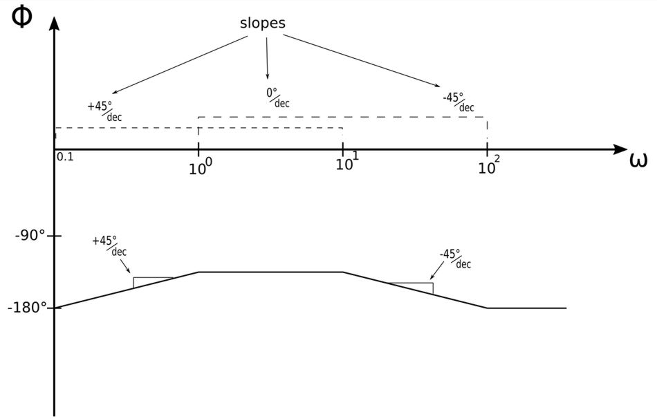
Notice how the imparted slope values for the simple zero and simple pole have ranges that overlap from 1-10 rad/sec. Within this frequency range, the slopes of both factors are combined (and in this case cancel each other out) giving:
- Phase plot slope from 1-10 rad/sec
- $$ = +45\frac{deg}{dec} + \Big(-45\frac{deg}{dec}\Big) = 0\frac{deg}{dec} $$
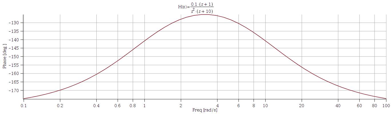
Exact Bode Phase Plot:
Below we see the exact Bode phase plot (achieved via software):
Continue on to Bode Plot (example #3)...