Sketch the Bode plots for the following transfer function:
$$ H(s) = \frac{s+3}{(s+2)(s^2+2s+25)} $$
Rewrite the expression in a recognizable form for zeros and poles:
We recognize that the transfer function contains a simple pole, simple zero and a quadratic/complex pole. We begin by rewriting the transfer function in a more standard form: $$ H(s) = \frac{3(1+\frac{s}{3})}{2(1+\frac{s}{2})25(\frac{s^2+2s+25}{25})}$$ $$ \qquad \; = \frac{0.06(1+\frac{s}{3})}{(1+\frac{s}{2}) \Big[ 1+\frac{2s}{25}+\frac{s^2}{25} \Big]} $$
$$ H(s) = \frac{0.06(1+\frac{s}{3})}{(1+\frac{s}{2}) \Big[ 1+\frac{0.4s}{5}+\Big(\frac{s}{5}\Big)^2 \Big]} \qquad,(Eqn\;1)$$
Determing magnitude via logarithms
If we substitute "jw" for "s" in equation #1 we get: $$ \mathbb{H}(j\omega) = \frac{0.06(1+\frac{j\omega}{3})}{(1+\frac{j\omega}{2}) \Big[ 1+\frac{0.4j\omega}{5}+\Big(\frac{j\omega}{5}\Big)^2 \Big]} $$ $$ \qquad \;\;\; = \frac{0.06(1+j0.333\omega)}{(1+j0.5\omega) ( 1-0.04\omega^2+j0.08\omega )} \qquad,(Eqn\;2) $$ Recall that the gain/magnitude of a transfer function is defined as: $$ H_{dB} = 20 \log_{10}|\mathbb{H}(j\omega)| $$ If we apply this expression to equation #2 and use the properties of logarithms we get the following expression:
$$ H_{dB} = 20\log_{10}0.06 + 20\log_{10}|1+j0.333\omega|-20\log_{10}|1+j0.5\omega|$$ $$\qquad \qquad \qquad \qquad -20\log_{10}|1-0.04\omega^2+j0.08\omega| $$ $$ H_{dB} = -24.4 +20\log_{10}(1+0.111\omega^2)^{\frac{1}{2}}$$ $$\qquad \qquad \qquad \qquad -20\log_{10}(1+0.25\omega^2)^{\frac{1}{2}}-20\log_{10}[(1-0.04\omega^2)^2+0.0064\omega^2]^{\frac{1}{2}} $$
$$ H_{dB} = -24.4 +10\log_{10}(1+0.111\omega^2)-10\log_{10}(1+0.25\omega^2)$$ $$\qquad \qquad \qquad \qquad -10\log_{10}[(1-0.04\omega^2)^2+0.0064\omega^2] $$
Sketch the magnitude plot by examining equation #1
By comparing equation #1 to the forms we derived for the Simple Zero, Simple Pole and quadratic pole, we see that we have the following corner frequencies: $$ \omega_0 = -2, +3, -5$$ ...where the "+" and "-" are simply a means of designating a zero (positive sign) and a pole (negative sign). We sketch the magnitude plot by examining each of the transfer function factors in order of increasing corner frequencies.
First Factor (constant term):
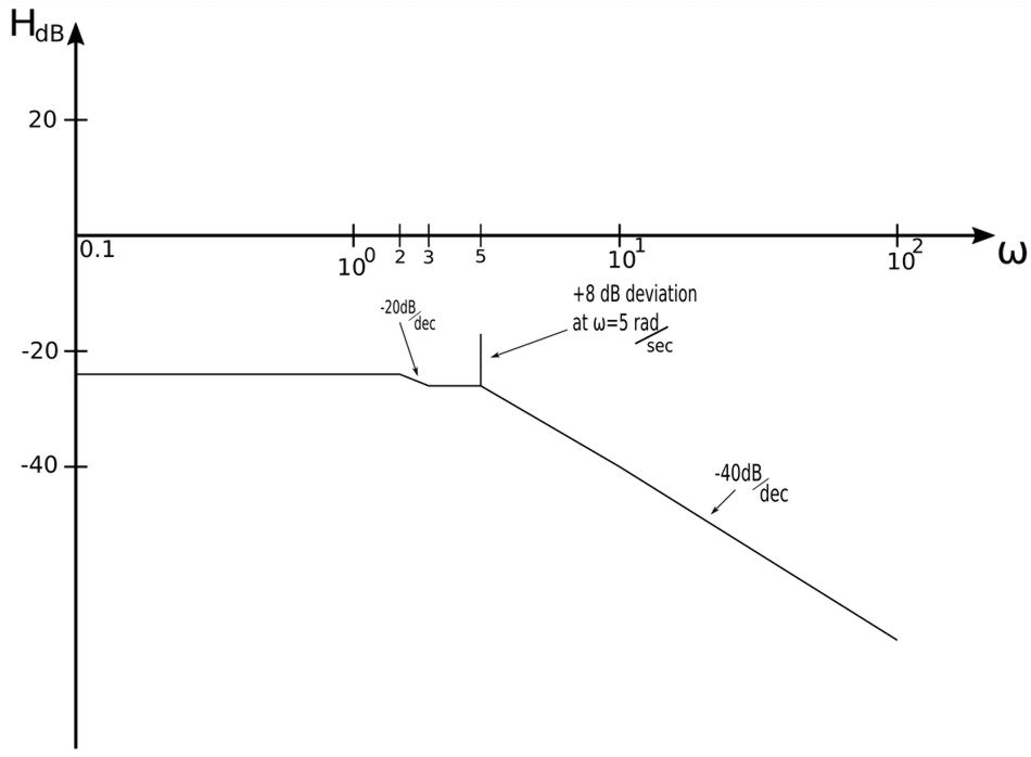
In equation #1 we see that the first factor is the constant 0.06. Recalling the section on Bode plots and constant factors, we know that the magnitude for the constant factor in our transfer function is: $$ H_{db} = 20\log_{10}0.06 = -24.4 dB $$ Since our transfer function contains no zeros or poles at the origin, our starting magnitude is -24.4 dB. We proceed to draw a straight horizontal line (slope=0 for constants) from the beginning of our plot (at 0.1 rad/sec) until the first corner frequency of 2 rad/sec. $$ H_{db} = -24.4 dB \qquad,(0.1 \leq \omega \leq 2) $$
Second Factor (simple pole):
The corner frequency of 2 rad/sec is associated with the Simple Pole: $$ \frac{1}{1+\frac{s}{2}} $$ The straight-line magnitude plot of a simple pole has a slope of -20dB/decade. Since the previous slope (for the constant) is 0, we plot a straight line with a slope of -20 dB/decade from 2rad/sec until we hit the next corner frequency of 3 rad/sec. $$ slope = -20\frac{dB}{dec} \qquad,(2 \leq \omega \leq 3)$$
Third Factor (simple zero):
The corner frequency of 3 rad/sec is associated with the Simple Zero: $$ 1+\frac{s}{3} $$ The straight-line magnitude plot of a simple zero has a slope of 20 dB/decade but this is combined with the previous slope of -20 dB/decade. This gives us a net slope of 0 dB/decade from 3 rad/sec to the next corner frequency (5 rad/sec): $$ slope = \Big( -20\frac{dB}{dec} + 20\frac{dB}{dec}\Big) = 0\frac{dB}{dec} \qquad,(3 \leq \omega \leq 5)$$
Fourth Factor (quadratic pole):
The corner frequency of 5 rad/sec is associated with the quadratic pole: $$ \frac{1}{1+\frac{0.4s}{5}+\Big(\frac{s}{5}\Big)^2} $$ The straight-line magnitude plot of a quadratic pole has a slope of -40 dB/decade and this is combined with the previous slope of 0 dB/decade. This gives us a net slope of -40 dB/decade from 5 rad/sec onward: $$ slope = \Big( -40\frac{dB}{dec} + 0\frac{dB}{dec}\Big) = -40\frac{dB}{dec} \qquad,(\omega \gt 5\frac{rad}{s})$$
Deviation at 5 rad/sec:
If you recall our discussion of Bode plots for quadratic poles and quadratic zeros of the transfer function, we mentioned how the damping coefficient (zeta) can be used to give more precision to the Bode magnitude plot. Specifically, at the corner frequency of our simple pole, the deviation between the straight-line magnitude plot and the actual plot can be defined as: $$ H_{deviation \; in \; dB} = -20\log_{10}(2\zeta) $$ Compare our quadratic pole: $$ \frac{1}{1+\frac{0.4s}{5}+\Big(\frac{s}{5}\Big)^2} $$ ...to the standard form for a quadratic pole: $$ \frac{1}{1+2\zeta\Big(\frac{s}{\omega_0}\Big)+\Big( \frac{s}{\omega_0} \Big)^2} $$ By equating terms, we see that for our pole, the following expression holds true: $$ 2\zeta = 0.4 \qquad,(where\;\zeta=damping\;coefficient) $$ We can now calculate the deviation at the corner frequency of 5 rad/sec: $$ H_{deviation \; @ \; \omega=5} = -20\log_{10}(2\zeta) $$ $$ \qquad \qquad \qquad \; = -20\log_{10}0.4 $$ $$ \qquad \qquad \qquad \; = +8.15 \; dB $$ We can represent this difference between the approximate and actual plot by drawing a vertical line at 5 rad/sec that goes upward 8.15 dB from the straight-line approximation. A smooth-curve line could then be drawn to better approximate the magnitude plot.
Straight-line approximation for Bode magnitude plot:
After examining the four factors of the transfer function in the manner described above, (and the deviation at the 5 rad/sec corner frequency) the final straight-line approximation of the Bode magnitude plot appears as follows
Exact Bode Magnitude Plot:
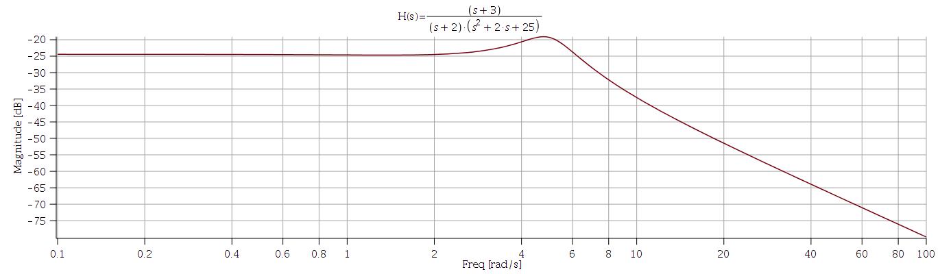
Below we see the exact Bode magnitude plot (achieved via software). Notice the upward "bump" at omega=5 rad/sec:
Determine phase using concept of phasors
Recall equation #2: $$ \mathbb{H}(j\omega) = \frac{0.06(1+j0.333\omega)}{(1+j0.5\omega) ( 1-0.04\omega^2+j0.08\omega )} \qquad,(Eqn\;2) $$ Also, recall that we can determine the phase angle of any complex phasor quantity by recognizing that: $$ \phi = \tan^{-1} \Big( \frac{imaginary\;part}{real\;part} \Big) $$ Applying this to equation #2 gives us:
$$ \phi = \tan^{-1}(0.333\omega)-\tan^{-1}(0.5\omega)-\tan^{-1}\Big( \frac{0.08\omega}{1-0.04\omega^2} \Big)$$
For the above equation, don't forget about the signs of the real and imaginary parts of the quadratic pole as they apply to reference angles from 180 degrees.
Sketch the phase plot
Simple Pole
Once again, when sketching the phase plot, it is important to remember that for factors of the transfer function not at the origin, the slopes of those factors affect the overall plot over a range of frequency values starting at one decade before to one decade after their respective corner frequencies. Consider the corner frequency of 2 rad/sec associated with the Simple Pole of our transfer function: $$ \frac{1}{1+\frac{s}{2}} $$
- For corner frequency of 2 rad/s:
- $$ 1 \; decade \; before = 0.2 \frac{rad}{s} $$
- $$ 1 \; decade \; after = 20 \frac{rad}{s} $$
A single Simple Pole has a straight-line phase plot with a slope of -45 deg/decade. Therefore, the simple pole in our transfer function imparts a slope of: $$ -45\frac{deg}{dec} \qquad,over \; the \; range\;(0.2 \leq \omega \leq 20) $$
Simple Zero
Now we look at the corner frequency of 3 rad/sec associated with the Simple Zero of our transfer function: $$ 1+\frac{s}{3} $$
- For corner frequency of 3 rad/s:
- $$ 1 \; decade \; before = 0.3 \frac{rad}{s} $$
- $$ 1 \; decade \; after = 30 \frac{rad}{s} $$
A single Simple Zero has a straight-line phase plot with a slope of +45 deg/decade. Therefore, the simple zero in our transfer function imparts a slope of: $$ +45\frac{deg}{dec} \qquad,over \; the \; range\;(0.3 \leq \omega \leq 30 ) $$
Quadratic Pole
We now look at the corner frequency of 5 rad/sec associated with the quadratic pole of our transfer function: $$ \frac{1}{1+\frac{0.4s}{5}+\Big(\frac{s}{5}\Big)^2} $$
- For corner frequency of 5 rad/s:
- $$ 1 \; decade \; before = 0.5 \frac{rad}{s} $$
- $$ 1 \; decade \; after = 50 \frac{rad}{s} $$
A single quadratic pole has a straight-line phase plot with a slope of -90 deg/decade. Therefore, the quadratic pole in our transfer function imparts a slope of: $$ -90\frac{deg}{dec} \qquad,over \; the \; range\;(0.5 \leq \omega \leq 50 ) $$
Constant term
The constant factor of our transfer function is: $$ 0.06 $$ As explained in the section on Bode plots and constant factors, the constant term imparts a phase angle of zero degrees. Once again, you may be tempted to draw a horizontal line at 0 degrees from w=0 up till our first frequency of interest (w=0.2). Remember however that the horizontal axis is logarithmic and as such we never include w=0 on the plot. Instead we use 0.1 rad/sec as our starting point and draw a straight horizontal line at 0 degrees from w=0.1 to our first frequency of interest (w=0.2): $$ 0^{\circ} = starting\;phase (0.1 \leq \omega \leq 0.2) $$
The final straight-line approximation (with annotations) is shown below:
Straight-line approximation for Bode phase plot:
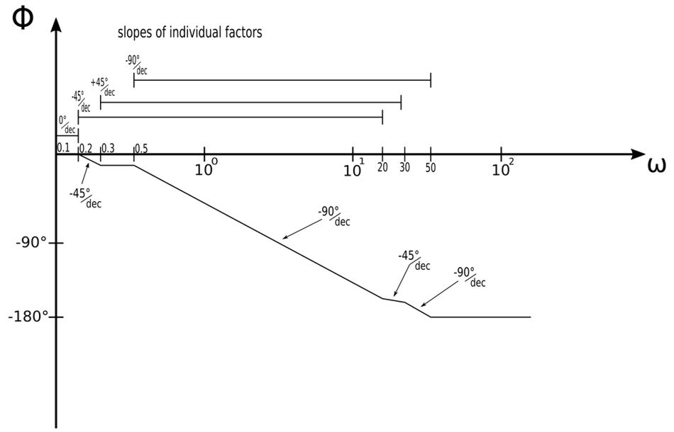
Notice how the imparted slope values for the individual factors have ranges that overlap. Within these overlapping frequency ranges, the slopes of those factors are combined.
Exact Bode Phase Plot:
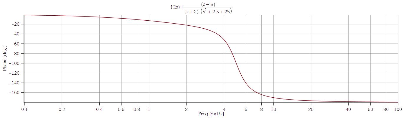
Below we see the exact Bode phase plot (achieved via software):
Continue on to Bode Plot (example #4)...