Sketch the Bode plots for the following transfer function:
$$ H(s) = \frac{0.2(10+s)}{s(2+s)} $$
Rewrite the expression in a recognizable form for zeros and poles:
By inspection you may see the the transfer function contains a pole at the origin, a simple zero and a simple pole. We begin by rewriting the transfer function as: $$ H(s) = 0.2 \Big[ \frac{10(\frac{10+s}{10})}{2s(\frac{2+s}{2})} \Big] $$
$$ H(s) = \frac{1+\frac{s}{10}}{s(1+\frac{s}{2})} \qquad,(Eqn\;1)$$
Determing magnitude via logarithms
If we substitute "jw" for "s" in equation #1 we get: $$ \mathbb{H}(j\omega) = \frac{1+\frac{j\omega}{10}}{j\omega(1+\frac{j\omega}{2})} $$ $$ \qquad \;\;\; = \frac{1+j0.1 \omega}{j\omega(1+j0.5\omega)} \qquad,(Eqn\;2)$$ Recall that the gain/magnitude of a transfer function is defined as: $$ H_{dB} = 20 \log_{10}|\mathbb{H}(j\omega)| $$ If we apply this expression to equation #2 and use the properties of logarithms we get the following expression: $$ H_{dB} = 20\log_{10}|1+j0.1\omega| - 20\log_{10}|j\omega| - 20\log_{10}|1+j0.5\omega| $$
$$ H_{dB} = 20\log_{10}\sqrt{1+0.01\omega^2} - 20\log_{10}\omega - 20\log_{10}\sqrt{1+0.25\omega^2} \qquad,(Eqn\;3) $$
Sketch the magnitude plot by examining equation #1
From equation #1 we see that we have the following corner frequencies: $$ \omega_0 = +10, -2 $$ ...where the "+" and "-" are simply a means of designating a zero (positive sign) and a pole (negative sign). We sketch the magnitude plot by examining each of the transfer function factors in order of increasing corner frequencies.
First Factor (pole at origin):
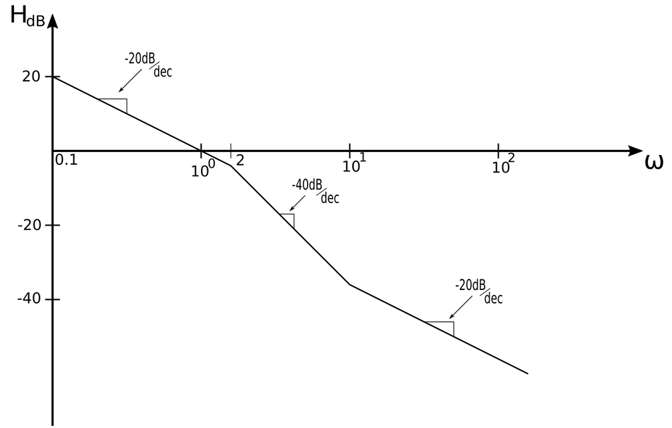
The first factor is a Pole at the Origin: $$ \frac{1}{s} $$ This means we start at 20dB and draw a straight line with a slope of -20dB/decade until we hit the first corner frequency of 2 rad/sec. $$ slope = -20\frac{dB}{dec} \qquad,(0 \leq \omega \leq 2)$$
Second Factor (simple pole):
The corner frequency of 2 rad/sec is associated with the Simple Pole: $$ \frac{1}{1+\frac{s}{2}} $$ The straight-line magnitude plot of a simple pole has a slope of -20dB/decade, but this is combined with the previous slope of -20dB/decade from the pole at the origin. This gives us a net slope of -40dB/decade in between the corner frequencies: $$ slope = \Big( -20\frac{dB}{dec} - 20\frac{dB}{dec}\Big) = -40\frac{dB}{dec} \qquad,(2 \leq \omega \leq 10)$$ Therefore we draw a straight line with a slope of -40dB/decade from 2 rad/sec to the next corner frequency (10rad/sec).
Third Factor (simple zero):
The corner frequency of 10 rad/sec is associated with the Simple Zero: $$ 1+\frac{s}{10} $$ The straight-line plot of a simple zero has a slope of +20dB/decade, but this is combined with the slope of the line we just drew for the simple pole. $$ slope = \Big( -40\frac{dB}{dec} + 20\frac{dB}{dec}\Big) = -20\frac{dB}{dec} \qquad,(\omega \gt 10\frac{rad}{s})$$
Straight-line approximation for Bode magnitude plot:
After examining the three factors of the transfer function in the manner described above, the final straight-line approximation of the Bode magnitude plot appears as follows
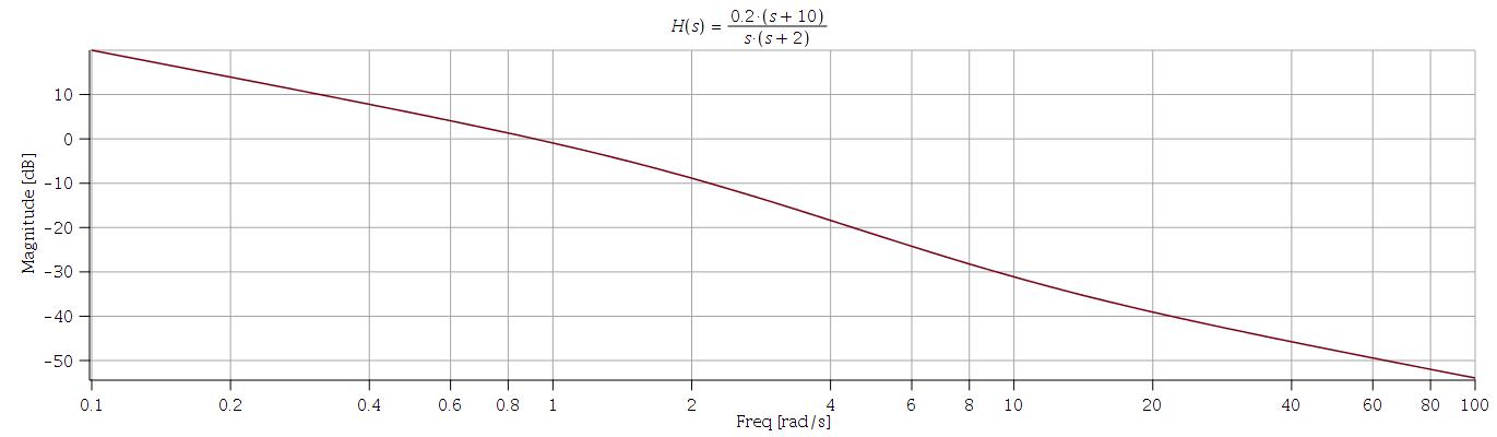
Exact Bode Magnitude Plot:
Below we see the exact Bode magnitude plot (achieved via software):
Determine phase using concept of phasors
Recall equation #2: $$ \mathbb{H}(j\omega) = \frac{1+j0.1 \omega}{j\omega(1+j0.5\omega)} \qquad,(Eqn\;2) $$ Also, recall that we can determine the phase angle of any complex phasor quantity by recognizing that: $$ \phi = \tan^{-1} \Big( \frac{imaginary\;part}{real\;part} \Big) $$ Applying this to equation #2 gives us:
$$ \phi = \tan^{-1}(0.1\omega) - 90^{\circ} - \tan^{-1}(0.5\omega) $$
Sketch the phase plot
Simple Pole
When sketching the straight-line phase plot, it is important to understand that for factors of the transfer function not at the origin, the slopes of those factors affect the overall plot over a range of frequency values starting at one decade before to one decade after their respective corner frequencies. For example, let's look at the corner frequency of 2 rad/sec associated with the Simple Pole of our transfer function: $$ \frac{1}{1+\frac{s}{2}} $$
- For corner frequency of 2 rad/s:
- $$ 1 \; decade \; before = 0.2 \frac{rad}{s} $$
- $$ 1 \; decade \; after = 20 \frac{rad}{s} $$
A single Simple Pole has a phase plot with a slope of -45 deg/decade. Therefore, the simple pole in our transfer function imparts a slope of: $$ -45\frac{deg}{dec} \qquad,over \; the \; range\;(0.2 \leq \omega \leq 20) $$
Simple Zero
Now consider the corner frequency of 10 rad/sec associated with the Simple Zero of our transfer function: $$ 1+\frac{s}{10} $$
- For corner frequency of 10 rad/s:
- $$ 1 \; decade \; before = 1 \frac{rad}{s} $$
- $$ 1 \; decade \; after = 100 \frac{rad}{s} $$
A Simple Zero has a phase plot with a slope of +45 deg/decade. Therefore, the simple zero in our transfer function imparts a slope of: $$ +45\frac{deg}{dec} \qquad,over \; the \; range\;(1 \leq \omega \leq 100) $$
Pole at the Origin
Now consider the Pole at the Origin for our transfer function: $$ \frac{1}{s} $$ The phase plot for a pole at the origin is a constant -90 degrees. Therefore, starting at the origin, we draw a straight line with zero slope at 90 degrees from the origin up until one decade below the first corner frequency we encounter. In our transfer function, the first corner frequency is 2 rad/s. One decade before that is 0.2 rad/s.
The final straight-line approximation (with annotations) is shown below:
Straight-line approximation for Bode phase plot:
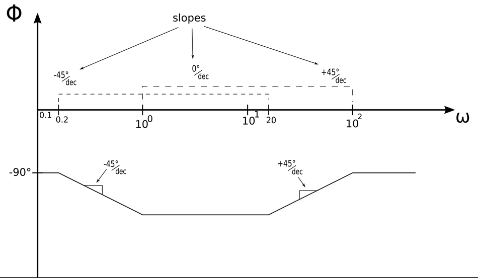
Notice how the imparted slope values for the simple zero and simple pole have ranges that overlap from 1-20 rad/sec. Within this frequency range, the slopes of both factors are combined (and in this case cancel each other out) giving:
- Phase plot slope from 1-20 rad/sec
- $$ = -45\frac{deg}{dec} + 45\frac{deg}{dec} = 0\frac{deg}{dec} $$
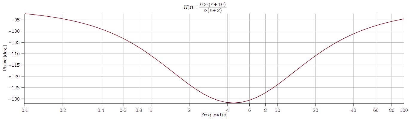
Exact Bode Phase Plot:
Below we see the exact Bode phase plot (achieved via software):
Continue on to Bode Plot (example #2)...